


Similarity condition
A comparative analysis of dissolution profiles between two medicinal products should take into account the similarity conditions. These include: comparison of mean values across time points with a recommended difference of no more than 10%, comparison of variation in results across time points with an acceptable lower variation for the test product and comparison of shape of the dissolution profile curves indicating similar dissolution mechanism.
Similarity criterion
To verify the similarity conditions, it is necessary to define the method and criterion for comparing dissolution profiles, ensuring that they adhere to principles of statistical validity. This process involves formulating a statistical hypothesis to determine the equivalence of dissolution profiles. The null hypothesis (H0) assumes that the release profiles are not similar, while the alternative hypothesis (Ha) proposes that the profiles of both products are similar. Therefore, the study's objective is defined by the alternative hypothesis. When testing these statistical hypotheses, it is important to understand the probability of making an incorrect decision about the similarity of profiles (Type I error, patient risk) and the probability of making an incorrect decision about the lack of similarity (Type II error, manufacturer risk). From the regulatory perspective, the main concern remains the false positive similarity conclusion. Therefore the selection of a similarity criterion needs to be driven by reduction of patient risk.
Method selection scheme
Regulatory agencies provide and general guidelines on the methods and principles for comparing in vitro dissolution profiles. The appropriate method for comparing dissolution profiles can be selected using the scheme outlined below. This scheme is proposed based on practical considerations and is not intended to cover all possible scenarios.
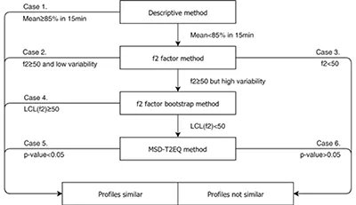
Descriptive method (Case 1)
The descriptive method is applicable for immediate release oral dosage forms with systemic action, where more than 85% of the drug is released from the dosage form at physiological pH within 15 minutes before gastric emptying (the mean gastric emptying half time T50%=15-20min). The product behaves like a solution and generally should not have any bioavailability problems. When reporting dissolution profiles comparison, it is sufficient to provide individual results of the percentage dissolved at the different sampling times pre-defined in the protocol and mean percentage dissolved with its variability (CV (%)) as well as a plot comparing the dissolution profiles of the test and reference products. If the mean dissolution value is higher than 85% in 15min for the reference and test product, the dissolution profiles can be considered similar without further statistical evaluation. However, it should be noted that the discriminatory power of the analytical method is necessary to demonstrate its capability in determining inter- and intra-batch variability and in identifying differences between the test and reference products.
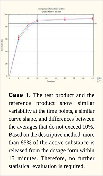
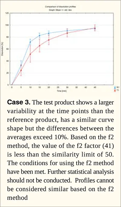
Similarity factor f2 method (Case 2, 3)
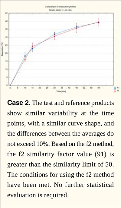
The method is based on determining the average Euclidean distance between the mean values of the reference product and the test product. Dissolution profiles can be considered similar if the f2 factor (rounded up to unity) is greater than 50, which corresponds to a 10% difference between the average values at each time point. The f2 method accounts for similarity by comparing mean values but does not consider variability at individual time points or differences in the shape of the release curve. It also does not control for type I error. Despite concerns regarding its statistical validity, simulation studies indicate that the f2 method is highly effective in detecting differences between profiles when the 10% threshold is exceeded, provided the prerequisites for its applicability are met. The method is recommended by all regulatory agencies, although there are minor differences in guidelines.
Similarity factor f2 bootstrap method (Case 4)
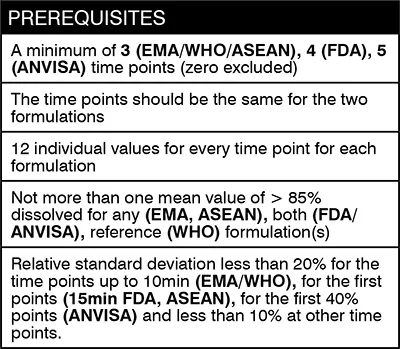
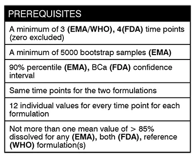
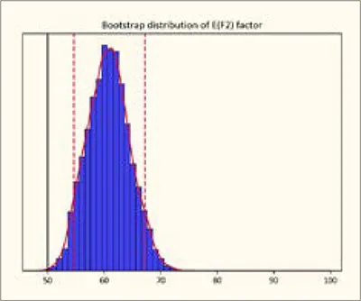
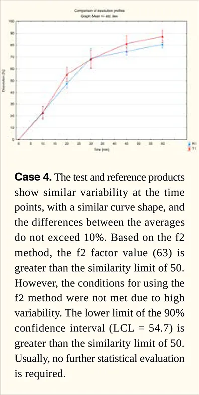
The similarity factor, calculated from a random sample of 12 units of the test and reference products, is a point estimate of the true f2 value for the population and varies from sample to sample. This estimator is biased, with the systematic error increasing as the variability in dissolution results increases. In cases of high variability in dissolution results that do not meet the conditions for applying the f2 similarity factor, the f2 procedure becomes ineffective. To statistically assess the compliance of the similarity factor with the similarity limit, it is necessary to determine its variability range (confidence interval) and compare the lower bound of this range with the similarity limit. However, determining the distribution of the f̂2 statistic is complex and does not allow for the analytical calculation of a confidence interval. To overcome this, a non-parametric bootstrap method can be employed as recently recommended by the EMA agency.
The f2, exp bootstrap method accounts for similarity conditions by comparing mean values and variability at individual time points, and it controls for type I error. However, it does not consider correlations between time points or the shape of the dissolution curve. It can be conservative, as the similarity factor estimator proposed by the EMA is only asymptotically unbiased when the sample size approaches infinity. Prior to using this approach it is advisable to identify the root cause of the excessive variability, which may result from a single unit deviating from the rest of the data or the formation of clusters of six units from two separate analysis runs as a result of poor experimental design. Although the method is recommended (EMA) in cases of excessive variability, the regulatory authority may request a justification for this variability, may ask for the bootstrap method to be supplemented with another method of assessing dissolution profiles, and may require a risk analysis of the impact of this variability on bioavailability.
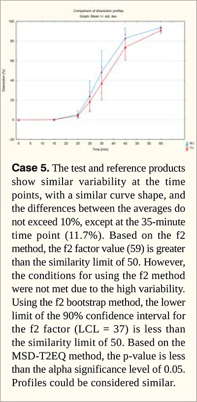
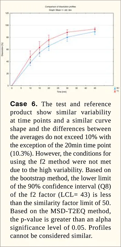
Multivariate statistical distance T2EQ method (Case 5, 6)
In cases of high variability in dissolution results, where the conditions for applying the f2 similarity factor are not met, the multivariate statistical distance (MSD-ACLMD) method, based on the approximate confidence limit of Mahalanobis distance (MD), was initially recommended. However, the EMA pointed out that, under certain assumptions, this method may indicate similarity between dissolution profiles even when differences in mean release values at individual time points exceed 10%. This limitation makes it undesirable for determining dissolution profile similarity, according to the EMA's recent stance. To address these concerns, the MSD-T2EQ method was proposed involving a comparison of Hotelling's T2 test statistic to a critical value determined based on the similarity limit, which corresponds to a 10% difference between the mean dissolution values standardised by a covariance matrix. The MSD-T2EQ method accounts for similarity conditions such as mean values, variability within and between individual time points, and ensures control over type I error. However, it does not consider the overall shape of the dissolution curve and shows low power in cases of intersecting profiles. This method can be applied in borderline cases where differences in mean values do not exceed 10%, but the conditions for using the f2 factor are not met, and high variability causes the lower limit of the confidence interval in the bootstrap method to fall below the similarity limit of 50. Notably, the method’s author does not restrict its use, emphasizing its statistical reliability from both regulatory and manufacturer perspectives, regardless of variability in dissolution results.
Highlights
• Carefully design the dissolution experiment to minimize sources of variability unrelated to the product.
• Review the specific requirements of each market for acceptable dissolution profile comparison methods, as minor differences exist.
• Apply the f2 similarity factor method when conditions for its use are met, as it is recommended by all regulatory agencies and is effective at detecting differences between profiles.
• Investigate the root cause of high variability in dissolution results before considering methods other than f2.
• Use the bootstrap method in cases of high variability in dissolution results according to recent recommendations by the EMA.
• In borderline cases, consider the multivariate statistical method MSD-T2EQ, which addresses the EMA's concerns regarding the MSD-ALCMD method.
References
1. European Medicines Agency EMA, 2010. Guideline on the investigation of bioequivalence. CPMP/EWP/QWP/1401/98 Rev. 1/ Corr **.
2. U.S. Department of Health and Human Services—Food and Drug Administration, CDER (FDA). Guidance for Industry - Dissolution Testing of Immediate Release Solid Oral Dosage Forms. 1997.
3. WHO Expert Committee on Specifications for Pharmaceutical Preparations: Annex 7 (WHO Technical Report Series, No. 992).
4. ASEAN, Guideline for the conduct of bioequivalence studies.
5. European Medicines Agency EMA, 2023. Clinical pharmacology and pharmacokinetics: questions and answers. p. 3.9,11,13.
6. European Medicines Agency, 2021. Reflection paper on statistical methodology for the comparative assessment of quality attributes in drug development (EMA/CHMP/138502/2017).
7. Moore JW, Flanner HH. Mathematical comparison of dissolution profiles. Pharm Technol. 1996; 20:64-74.
8. Shah, V. P.; Tsong, Y.; Sathe, P.; Liu, J. P. In Vitro Dissolution Profile Comparison—Statistics and Analysis of the Similarity Factor, f2. Pharm. Res. 1998, 15 (6), 889–896.
9. M.-C. Ma, B.B.C. Wang, J.-P. Liu, Y. Tsong. Assessment of similarity between dissolution profiles., J Biopharm Stat. 10 (2000) 229–249.
10. Hoffelder T. Equivalence analyses of dissolution profiles with the Mahalanobis distance. Biom J. 2019; 61(5):1120–37.
11. https://dpc.statsoftpharma.eu/